5 Compound Interests and the Time Value of Money
Chapter Five Learning Objectives
- Define opportunity cost and the time value of money.
- Understand how compound interests work.
- Define future value and perform future value calculations.
- Define present value and perform present value calculations.
- Define annuity and perform annuity calculations.
- Apply time value of money concepts to inflation, investment returns, interest on borrowing, and personal financial planning.
- Distinguish different types of interest rates.
- Identify key economic and political factors affecting interest rates.
“A dollar today is worth more than a dollar tomorrow.” You may have heard this saying before. Do you agree? How would you explain your answer?
Opportunity Cost
Before we continue, it is useful to first explore a concept called opportunity cost. Everyday you make decisions that have opportunity costs that you may or may not be aware of. Consider the following choices:
| Have taco for lunch or…… | have pizza for lunch? |
| Take a nap or…… | go for a run? |
| Work extra shifts or…… | take a vacation trip over spring break? |
Economists define opportunity cost as the value of the next-best alternative when you make a decision. Assuming your appetite is limited, the opportunity cost of eating pizza for lunch is having tacos. It is what you give up when you choose one alternative over another. What is the opportunity cost of going for a run? In this case, it is taking a nap. People often overlook opportunity costs when making decisions. The cost of vacationing over spring break is not just the cost of the trip. The amount of money you could make by working extra shifts is the opportunity cost of the vacation and should be part of your decision. Opportunity costs play an important role in personal finance.
Let us look at the saying again. If you do not spend a dollar today, you can invest the dollar. We will use the terms rate of return or return to describe earnings from an investment. The expected return on an investment is positive because no one will invest in something that is expected to lose money. Expected return is not the same as realized return, which is the actual return and may be positive or negative. Another reason expected return is positive is due to inflation, which is defined as the increase in the price of goods and services over time. For example, you want to buy a new bicycle, which costs $400 today. If you wait one year, the price of the same bicycle goes up to $450. If the return on investing the $400 is less than $50, you will be better off buying the bicycle today. This is before taking into account the opportunity costs of not being able to use the bike during that time. To entice consumers to invest, the expected return on an investment must account for inflation.
Since you can earn a return on your investment, the dollar you invest today is expected to grow to more than one dollar in the future. The opportunity cost of spending a dollar today is the return you expect to earn by investing it. Therefore, a dollar today is worth more than a dollar tomorrow. We call this the time value of money and it is a core concept in finance. Time value of money calculations are fundamental tools for analyzing investments, loans, and financial planning. You can apply these tools to determine how much you need to save each month to reach a particular financial goal, such as making down payment on a house. Mastering these concepts will enable you to understand and compare different investment and loan options. With this knowledge, you will make better financial decisions.
Example: Jordan learning about time value of money
Jordan is 24 years old and recently graduated from college. They are learning about personal finance and developing a personal financial plan. After putting together a budget, they found that they can save $10 per day by preparing breakfast and lunch at home. It will also save them time from driving to pick up these meals and have more free time in the morning and during lunch break. Even though $10 does not seem like a lot of money, Jordan feels that is a goal they can achieve. They are surprised to learn that by investing $300 per month ($10 per day x 30 days) and earning 8 percent per year on their investment, these savings can grow to over $1 million in 40 years!
Understanding Compounding
In the world of finance, compounding refers to the process where the return earned or interest owed is added back to the investment or loan. This continuous reinvestment allows the balance to grow and accumulate over time. This phenomenon is also referred to as “interest on interest.”
The snowball effect is the best way to see how powerful compounding can be. Each time the return is reinvested, the snowball gets bigger, picking up even more snow in the next round. The longer you invest, the more you earn, which means the amount you earn each period gets larger and larger. With compounding, your investment grows faster and bigger over time. Unfortunately, the same is true for the loan balance if you do not make any payments and let interest accumulate.
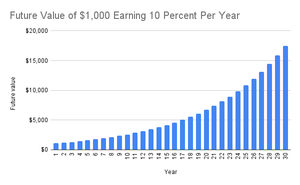
To illustrate how compounding works, let us look at an investment that earns 10 percent per year. If you put $1,000 into this investment, how much would you earn in one year? over two years? over 30 years?
Your earnings after one year would be $100 ($1,000 x 0.10). If you extrapolate earnings over two years to be $200 ($100 x 2) and earnings over 30 years to be $3,000 ($100 x 30), your calculation implicitly assumes simple interest. This means earnings are not reinvested.
With compounding, your earnings will grow year after year and at an increasing rate.
Year One: Your earning after one year would also be $100 ($1,000 x 0.10). However, the new balance after reinvesting is $1,100 ($1,000 + $100).
Year Two: In the second year, the return is based on the new balance of $1,100, resulting in $110 ($1,100 x 0.10). The balance after two years is $1,210 ($1,100 + $110). Notice how your earning in the second year, $110, is greater than that in the first year, $100, because of compounding. Over two years, you earn $210 ($110 + $100).
Year Three and Beyond: This pattern continues each year and over 30 years you would earn about $16,450 in return and your investment would have an ending balance of $17,450, significantly more than what you would earn without compounding (simple interest).
Your earnings increase each year because you make money not only on your original investment but also on the accumulated earnings from previous years. This is the essence of compounding – your money earns money, and over time, this leads to significant growth. Figure 5.1 shows the effects of compounding as the investment horizon lengthens. The term future value refers to the ending balance of the investment.
How much your money grows depends on a number of factors. The first factor is time. The longer you invest, the more your money grows. Secondly, the higher the rate of return on an investment, the more your money grows. Finally, the more often you reinvest, the more your money grows. This last factor is called compounding frequency, which is defined as the number of times in a year interest or return is computed and added to the balance. Hence, annual compounding means once per year. Monthly compounding means 12 times per year. Quarterly compounding means 4 times per year, etc. Many consumer loans such as credit cards, auto loans, and mortgages have monthly compounding. If you do not make the scheduled monthly payment, any unpaid amount is added to the loan balance, increasing future interest. Some people are surprised to find that even if they do not make new purchases, their credit card balances continue to grow rapidly. To be an informed consumer, you will want to know how the credit card companies and banks determine your payments. The next topic in this chapter, time value of money calculations, will address these questions.
Time Value of Money Calculations
As noted in the last section, the relationship between time and money depends on a number of factors. We use the term present value (PV) to describe the value at the beginning of an investment horizon. It is also the value of a loan’s initial amount. Future value (FV) refers to the value at the end of an investment horizon or the final balance of a loan. Before going over how to use a spreadsheet to perform time value of money calculations, it is useful to examine the basic time value of money formula.
Future Value = Present Value x (1 + rate of return)Investment Horizon
Let us look at the $1,000 investment that earns 10 percent per year again. The present value of this investment is $1,000. The rate of return is, of course, 10 percent. The future value of this investment can be determined using the above formula.
- Future value of $1000 after one year = $1,000 x (1 + 0.1)1 = $1,100
- Future value of $1000 after two years = $1,000 x (1 + 0.1)2 = $1,210
- Future value of $1000 after 30 years = $1,000 x (1 + 0.1)30 = $17,449
You can see that this “formula” is simply a short-cut for computing the future value with reinvested earnings. Earlier we indicated that the longer you invest, the more your money grows. You just verified that this claim is true with your own calculations. Your investment after 30 years is worth a lot more than after just 2 years. The ability to confirm theories with numerical examples is a great feature of many finance concepts. Next, let us look at the effect of different rates of return on an $1,000 investment over 30 years.
- Future value of $1000 after 30 years at 4 percent = $1,000 x (1 + 0.04)30 = $3,243
- Future value of $1000 after 30 years at 8 percent = $1,000 x (1 + 0.08)30 = $10,063
- Future value of $1000 after 30 years at 12 percent = $1,000 x (1 + 0.12)30 = $29,960
The above results confirm that the higher the rate of return, the more your money grows. The future value of an investment is positively related to the length of time and the rate of return on the investment. In other words, the longer the investment horizon and the higher the rate of return, the larger will the future value be.

The basic time value of money formula is relatively simple, yet it has many applications. Some of you may recognize that it has the same form as the exponential growth formula. We can use it to estimate the effect of inflation on prices by using the rate of inflation as the rate of return. You may have come across old photos showing prices from decades ago. Everything seems to be so much cheaper back then. Figure 5.2 is an excerpt from a grocery store flyer in 1985 advertising bread for 99 cents and a pound of bananas for 39 cents. The inflation rate averaged 2.83 percent per year between 1985 and 2025 according to the Bureau of Labor Statistics. What would the inflation adjusted prices be for these items 40 years later in 2025?
- Price of bread after 40 years at an inflation rate of 2.83 percent = $0.99 x (1 + 0.0283)40 = $3.02
- Price of bananas after 40 years at an inflation rate of 2.83 percent = $0.39 x (1 + 0.0283)40 = $1.19
Example: Estimating future cost of college
Accounting for the effect of inflation is especially important when evaluating long-term financial goals. For instance, a couple is saving for their newborn child’s college education. Currently the average cost of a state university is around $12,000 per year. The cost of college has increased by 5 percent per year on average over the past decade. Assuming this trend continues, they will need more than $12,000 per year when their child enters college. But how much more? They can get an estimate of how much the future cost would be by applying time value of money calculations.
- Time horizon: 18 years
- Rate of increase: 5 percent per year
- Current cost of college: $12,000
Future Cost of college after 18 years = $12,000 x (1 + 0.05)18= $28,879
Exercise 5.1: Inflation adjusted prices
- The average price of gasoline per gallon was $1.12 in 1985. Using an average inflation rate of 3 percent per year, what would the inflation adjusted price be for gasoline today? How does the current price you see at gas stations compare to your calculated inflation adjusted price?
- The federal minimum wage in the United States in 1985 was $3.35 per hour. If the minimum wage were to increase at the rate of inflation at 3 percent per year, what would the inflation adjusted minimum wage be today? Look up the current federal minimum wage. How does it compare to your calculation?
While the basic time value of money formula is easy to use, it has some limitations. One is that it can only handle a single dollar amount, which is referred to as a lump sum cash flow in finance. A more common type of cash flow in everyday life is an annuity, which consists of multiple fixed dollar amounts that are received or paid at equal time intervals. An ordinary annuity has payments that occur at the end of each period. An annuity due has payments that occur at the beginning of each period. Auto loans and mortgages with fixed monthly payments are examples of ordinary annuities. Rent is an example of an annuity due because rent is usually due at the beginning of each month. To compute the future value of an annuity is not simple. In theory, you can compute the future value of each fixed payment in an annuity individually using the formula and then sum up the total. Such calculations become time consuming and tedious very quickly. Fortunately, spreadsheet software has built in functions to compute annuity and lump sum cash flows, simplifying time value of money calculations. Using these functions can provide useful answers to many financial planning questions.
Using A Spreadsheet to Perform Time Value of Money Calculations[1]
Spreadsheet software such as Google Sheets or Microsoft Excel have functions that can perform time value of money calculations, such as computing future value (FV), present value (PV), rate of return or interest rate per time unit (RATE), number of periods in the investment horizon or loan term (NPER), and annuity payment amount per time unit (PMT). We will go over each of these calculations and their applications in the following sections. It is important to pay attention to compounding frequency when using these built-in functions and ensure that the time unit matches. For instance, if a loan requires monthly payments, then the number of periods should be the number of months and the rate of return should be the interest rate per month. Mismatches are easy to overlook because the information provided by banks and businesses is often stated in various time units. Interest rates are usually quoted as interest rates per year. Auto loan terms are often stated in months (36 months, 48 months, 60 months, etc.) and home mortgage terms are stated in years (15 years, 30 years). Since the mortgage requires monthly payments, you need to make adjustments accordingly so that interest rate and loan terms are stated in monthly units. To obtain the interest rate per month, divide the annual rate by 12 because there are 12 months in a year. The loan term for a 30 year mortgage is 360 months (30 years x 12 months per year). If you make checking the time unit the first step in your calculations, you are a lot less likely to overlook any mismatches.
| Spreadsheet function names | Output from function |
| FV() | Computes the future value (FV): the value at the end of an investment horizon or the final balance of a loan. The output is a dollar amount. |
| PV() | Computes the present value (PV): the value at the beginning of an investment horizon or the initial balance of a loan. The output is a dollar amount. |
| RATE() | Compute the rate of return or interest rate per period. The output is a decimal that is usually formatted as a percentage. |
| NPER() | Computes the number of periods in the investment horizon or loan term. The output is a time unit. |
| PMT() | Computes the annuity payment: a stream of cash flows in equal dollar amounts that are received or paid at equal time intervals. The output is a dollar amount. |
When the output of the function is a dollar amount (FV, PV, PMT), the result can be positive or negative. A positive value signifies that the cash flow is an inflow and a negative value signifies that the cash flow is an outflow. This is because the software assumes that cash flows in a time value of money calculation cannot all have the same sign (all positive or all negative). The software assumes that if you take out a loan today, you will receive the cash now (a cash inflow) and you will need to pay back interests and the borrowed money in the future (cash outflows). As a rule of thumb, the initial value of a loan is treated as a cash inflow and a present value. Loan payments and future ending balance are treated as cash outflows.
To use a spreadsheet to perform time value of money calculations, you need to input values into these functions. Google Sheets and Excel use different notations for these inputs. The following table provides descriptions for these input variables and their corresponding notations in Google Sheets and Excel. The next section will explain each function and include examples to illustrate how to use them.
| Description of input variables | Notation in Google Sheets | Notation in Excel |
| The rate of return (or interest rate, or growth rate, or inflation rate) per time unit. This input variable is a decimal. | rate | rate |
| The number of periods in the investment horizon or loan term. This input variable is a time unit. | number_of_periods | nper |
| The amount of annuity cash flow per time unit. This input variable is a dollar amount and can be positive or negative. | payment_amount | pmt |
| The current value of an investment or a loan. This input variable is a dollar amount and can be positive or negative. | present_value | pv |
| The future value of an investment or a loan. This input variable is a dollar amount and can be positive or negative. | future_value | fv |
| This input variable is an indicator for whether the annuity cash flows occur at the end or at the beginning of each period. Use 0 (or omit) if the annuity occurs at the end of each period, an ordinary annuity. Use 1 if the annuity occurs at the beginning of each period, an annuity due. The default, if it is left empty, assumes the annuity is an ordinary annuity with cash flows at the end of each period. | end_or_beginning | type |
Future Value Calculation
Future value calculations have many uses, as demonstrated in earlier sections in this chapter. It can be used to determine the future worth of an investment, the future balance of a loan, or the estimated future prices based on expected inflation. The spreadsheet function for computing future value is FV() and it requires five input variables: (1) the rate of return per time unit, (2) the number of periods in the investment horizon, (3) the amount of annuity cash flow per time unit, (4) present value, (5) an indicator for whether the annuity cash flows occur at the end or at the beginning of each period. To use a built-in function, start with an equal sign (=) before the function name. We will use several examples to demonstrate how to compute future values. Implement the calculations in these examples using your preferred spreadsheet software.
Future value function: FV()
| Google Sheets | FV(rate, number_of_periods, payment_amount, present_value, [end_or_beginning]) |
| Excel | FV(rate, nper, pmt, pv, [type]) |
Example: Future value of a lump sum investment
Jordan received $2,000 as a graduation gift today and decided to put the money into an Individual Retirement Account (IRA) and expects to earn 11 percent per year on this investment. Compute the estimated value of this investment after 40 years.
The time unit for this calculation is year. The $2,000 is the present value because it is the amount of money at the start. Treat this as a cash outflow and enter this amount as -2000. The rate of return is 11 percent per year and the number of periods is 40 years. There is no additional cash flow so the annuity amount is 0.
- rate: 0.11
- number_of_periods: 40
- payment_amount: 0
- present_value: -2000
- end_or_beginning: left blank
- Spreadsheet entry: =FV(.11, 40, 0, -2000)
- Result: $130,002
What would happen if you enter 2000 instead of -2000? Try it out!
- rate: 0.11
- number_of_periods: 40
- payment_amount: 0
- present_value: 2000
- end_or_beginning: left blank
- Spreadsheet entry: =FV(.11, 40, 0, 2000)
- Result: -$130,002
The spreadsheet software assumes that if one of the cash flows is an inflow, the other must be an outflow.
Example: Future value of constant regular investments
In a previous example, Jordan decided to save $300 per month by preparing breakfast and lunch at home. We claimed that by earning a return of 8 percent per year, these savings would grow to over $1 million in 40 years! Now you have the tools to check this claim.
The time unit of this calculation is month because Jordan is putting away money each month. The $300 per month is an annuity cash flow. Since this is money being put away, the amount is entered as a cash outflow (negative). The investment horizon is 480 months (40 years x 12 months per year). The rate of return per month is 8 percent divided by 12. There is no present value so the amount entered is $0. Jordan plans to invest the money at the end of each month so this is an ordinary annuity and the indicator variable can be left blank or 0.
- rate: 0.08/12
- number_of_periods: 480
- payment_amount: -300
- present_value: 0
- end_or_beginning: left blank
- Spreadsheet entry: =FV(.08/12, 480, -300, 0)
- Result: $1,047,302
How would the outcome change if Jordan waited 10 years before implementing this savings scheme? Assume that everything else remains the same, i.e. Jordan would put away $300 per month into an investment that earns 8 percent per year. The only difference is that the investment horizon would only be 360 months (30 years x 12 months).
- rate: 0.08/12
- number_of_periods: 360
- payment_amount: -300
- present_value: 0
- end_or_beginning: left blank
- Spreadsheet entry: =FV(.08/12, 360, -300, 0)
- Result: $447,108
Did the answer surprise you? Did you expect the future value to decrease by more than half by waiting 10 years?
Example: Future value of credit card balances
Before taking a personal finance course Sam had made some unwise spending decisions and had racked up $8,000 in credit card debt. The card carries a 24 percent interest rate per year and monthly minimum payment of $50. If Sam makes the minimum payment for 24 months and does not make any additional purchases, what will the future balance be at the end of the 24 months?
The time unit of this calculation is month. The $50 monthly minimum payment is an annuity cash flow. Since these are payments, Sam should treat them as cash outflows. The number of periods under consideration is 24 months. The interest rate is 2 percent per month (24 percent per year / 12 months). The credit card balance today is $8,000 and represents the present value in this calculation. This amount is considered a cash inflow because it is money Sam does not have to pay today. A general rule of thumb is to treat initial loan balance as a cash inflow. Payment for this credit card is due at the end of each month so the annuity is an ordinary annuity and the indicator variable can be left blank or 0.
- rate: 0.24/12
- number_of_periods: 24
- payment_amount: -50
- present_value: 8000
- end_or_beginning: left blank
- Spreadsheet entry: =FV(0.24/12, 24, -50, 8000)
- Result: -$11,346
The future value is negative, meaning this is the amount Sam needs to pay after 24 months. In this example, even though Sam stops making new purchases and makes the minimum payment, the balance on the credit card continues to grow. To unravel this mystery, let us look at how much interest is charged on the balance in the first month. Sam owes $8,000 and the credit card company charges 2 percent per month, meaning the company charges $160 ($8,000 x 0.02) in interest in the first month. The minimum payment of $50 is not sufficient to cover the interest charged and $110 ($160 – $50) will be added to the balance in the next month. This means the interest charge will be even higher next month and the process continues. The effect of compounding is at work again, this time against Sam.
Exercise 5.2: Compute Future Value
Use the spreadsheet function, =FV(), to compute future values. Compare your results to those in earlier sections of this chapter.
- Compute the future value of a $1,000 investment today that earns 10 percent per year in one year.
- Compute the future value of a $1,000 investment today that earns 10 percent per year over two years.
- Compute the future value of a $1,000 investment today that earns 10 percent per year over 30 years.
- Compute the future value of a $1,000 investment today that earns 4 percent per year over 30 years.
- Compute the future value of a $1,000 investment today that earns 8 percent per year over 30 years.
- Compute the future value of a $1,000 investment today that earns 12 percent per year over 30 years.
- Based on your own calculations, what relationship do you observe between investment horizon and future value? Between interest rate and future value?
Present Value Calculation
Present value calculation can be used to determine how much a series of annuity cash flows is worth today. The calculation can also estimate how much money to set aside today as a lump sum to reach a specific future goal. The process of computing present value is called discounting and the rate of return is often referred to as the discount rate. Present values are affected by the rate of return, the length of the time horizon, and the cash flow amount in the future. The higher the rate of return, the smaller the present value needed to reach the same future goal. Similarly, the longer the investment horizon, the smaller the present value needed. On the other hand, the larger the cash flow amount in the future, the larger the present value. Computing present value is one of the most commonly used methods in financial analysis because the value of an investment is the present value of its future cash flows. This method of valuing an investment is called discounted cash flow analysis.
The spreadsheet function for computing present value is PV() and it requires five input variables: (1) the rate of return per time unit, (2) the number of periods in the investment horizon, (3) the amount of annuity cash flow per time unit, (4) future value, (5) an indicator for whether the annuity cash flows occur at the end or at the beginning of each period. We will use several examples to demonstrate how to compute present values. Again, you should follow these examples using your preferred spreadsheet software.
Present value function: PV()
| Google Sheets | PV(rate, number_of_periods, payment_amount, future_value, [end_or_beginning]) |
| Excel | FV(rate, nper, pmt, fv, [type]) |
Example: Present value of a lump sum retention bonus
Jordan’s company offers a retention bonus of $15,000 if an employee stays with the firm for 3 years. A recruitment firm reached out to Jordan and a competitor is offering a sign-on bonus of $12,000 today. If Jordan were to receive the sign-on bonus, they can earn 8 percent per year by investing the money. Assuming all other attributes of the two jobs are the same, how can Jordan compare the sign-on bonus today versus the retention bonus in 3 years? One approach is to compute the present value of the retention bonus.
The time unit of this calculation is year. The retention bonus will be received 3 years from now. Therefore it is a cash inflow and a future value. The rate of return (discount rate) is 8 percent per year. There are no other cash flows.
- rate: 0.08
- number_of_periods: 3
- payment_amount: 0
- future_value: 15000
- end_or_beginning: left blank
- Spreadsheet entry: =PV(0.08, 3, 0, 15000)
- Result: -$11,907
The result of -$11,907 means that if Jordan were willing to put away $11,907 into an investment that earns 8 percent per year, that investment would grow to $15,000 in 3 years. In other words, the retention bonus of $15,000 in 3 years is worth only $11,907 today, slightly less than the $12,000 sign-on bonus.
Remember that present value is affected by the discount rate. How would the analysis change if the rate of return is 4 percent per year? or 12 percent per year?
- rate: 0.04
- number_of_periods: 3
- payment_amount: 0
- future_value: 15000
- end_or_beginning: left blank
- Spreadsheet entry: =PV(0.04, 3, 0, 15000)
- Result: -$13,335
- rate: 0.12
- number_of_periods: 3
- payment_amount: 0
- future_value: 15000
- end_or_beginning: left blank
- Spreadsheet entry: =PV(0.12, 3, 0, 15000)
- Result: -$10,677
This example demonstrates that present value decreases when the discount rate increases.
Example: Present value of constant regular cash flows
In learning about the competitor’s sign-on bonus, Jordan’s company is willing to change their retention bonus structure. Jordan will receive $5,000 each year for 3 years with the first payment at the end of year one. The rate of return is still 8 percent per year. Do you think this new structure is more valuable than the original one? Let us find out.
The time unit of this calculation is year. The retention bonuses will be $5,000 per year starting at the end of year one. Therefore it is a cash inflow and an ordinary annuity and the indicator variable can be left blank or 0. The rate of return (discount rate) is 8 percent per year. There is no future value.
- rate: 0.08
- number_of_periods: 3
- payment_amount: 5000
- future_value: 0
- end_or_beginning: left blank
- Spreadsheet entry: =PV(0.08, 3, 5000, 0)
- Result: -$12,885
The above calculations show that the present value of an annuity of $5,000 per year over 3 years is higher than the present value of a $15,000 lump sum received at the end of 3 years. This is because the $5,000 that Jordan receives at the end of year one and year two can be invested to earn an 8 percent return.
Exercise 5.3: Compute Present Value
Use the spreadsheet function, =PV(), to compute present values.
- Compute the present value today of an investment that promised $10,000 in one year when the discount rate is 10 percent per year.
- Compute the present value today of an investment that promised $10,000 in two years when the discount rate is 10 percent per year.
- Compute the present value today of an investment that promised $10,000 in 30 years when the discount rate is 10 percent per year.
- Compute the present value today of an investment that promised $10,000 in 30 years when the discount rate is 4 percent per year.
- Compute the present value today of an investment that promised $10,000 in 30 years when the discount rate is 8 percent per year.
- Compute the present value today of an investment that promised $10,000 in 30 years when the discount rate is 12 percent per year.
- Based on your own calculations, what relationship do you observe between investment horizon and present value? Between interest rate and present value?
Annuity Payment Amount Calculation
Many personal finance decisions require computing annuity payment. It can help you determine the amount of regular savings required to reach a financial goal. It can estimate the monthly payment on an auto loan or a mortgage.
The spreadsheet function for computing annuity payment amount is PMT() and it requires five input variables: (1) the rate of return per time unit, (2) the number of periods in the investment horizon, (3) present value, (4) future value, (5) an indicator for whether the annuity cash flows occur at the end or at the beginning of each period.
It is important to pay attention to whether the present value and future value are inflows or outflows. When analyzing loans, the initial amount borrowed is treated as the present value and a cash inflow. The resulting annuity payment amount from the spreadsheet function will be shown as negative, a cash outflow. We will use several examples to demonstrate how to use this function to analyze financial planning decisions.
Annuity payment amount function: PMT()
| Google Sheets | PMT(rate, number_of_periods, present_value, future_value, [end_or_beginning]) |
| Excel | PMT(rate, nper, pv, fv, [type]) |
Example: Annuity payment amount to reach a future financial goal
Sam was intrigued when Jordan shared that saving a few hundred dollars per month could grow to over $1 million in 40 years. Sam’s goal is to have $1,500,000 by age 70. Being relatively young at 25 years old, Sam is willing to take on more risk and plans to invest in the stock market and expects to earn 10 percent per year on average. How much will Sam need to save each month to reach this goal?
The time unit of this calculation is month. The $1,500,000 is future value and represents a cash inflow in 45 years (age 70 – age 25). Since the time unit is month, the investment horizon is 540 months (45 years x 12 months). The rate of return is 10 percent divided by 12. Sam has no current savings so the present value is $0. Since Sam will put aside savings at the end of each month, the savings will be an ordinary annuity and the indicator variable should be left blank or 0.
- rate: 0.10/12
- number_of_periods: 540
- present_value: 0
- future_value: 1500000
- end_or_beginning: left blank
- Spreadsheet entry: =PMT(0.10/12, 540, 0, 1500000, 0)
- Result: -$143
The analysis shows that Sam only needs to save $143 per month to reach the goal of $1,500,000 in 45 years assuming the rate of return is 10 percent per year. How much would Sam need to save to reach the same goal if they wait until age 40 to begin saving?
If Sam waits until age 40, there will only be 30 years (360 months) left to save. The calculation is the same except the investment horizon (number_of_periods) is now 360.
- Spreadsheet entry: =PMT(0.10/12, 360, 0, 1500000, 0)
- Result: -$664
This example illustrates the importance of saving early! Even if the amount is relatively small, the power of compounding has a great impact.
Example: Auto loan and auto lease payments (Note: we will discuss automobile purchase in detail in a later chapter. This example examines a simplified scenario. )
A car dealer is offering two financing options on a car selling for $32,000. The first option is to purchase the car with a 36-month loan at 9 percent per year. The second option is to lease the car. Assume that the buyer will put $2000 as down payment. First, compute the monthly payment for buying this car.
Since the car sells for $32,000, with a $2,000 down payment, the buyer needs to borrow $30,000 ($32,000 – $2,000). The time unit is month. The interest rate is 9 percent divided by 12 and the loan term is 36 months. The auto loan must be fully paid off after 36 months so the future value is $0. The monthly payment is due at the end of each month.
- rate: 0.09/12
- number_of_periods: 36
- present_value: 30000
- future_value: 0
- end_or_beginning: left blank
- Spreadsheet entry: =PMT(0.09/12, 36, 30000, 0, 0)
- Result: -$954
The monthly payment on this auto loan is $954. When the buyer indicates that this amount is too high, the dealer offers a lease option with monthly payment of $320. That is a huge difference. How did the dealer do that?!?
There are a few important differences between buying and leasing and we will discuss those in detail in a later chapter. One critical difference is that the consumer does not own the car at the end of a lease. The estimated future value of the car at the end of the lease plays a key role in reducing the monthly payment. The dealer in this example estimates the car will be worth $26,000 at the end of the 36 month lease after adjusting for inflation. If the consumer wants to own the car, they would need to pay $26,000 at the end of the lease. The time value of money calculation for the lease will include the $26,000 as a cash outflow in future value. Unlike auto loans, car lease payments are typically due at the beginning of each month, which makes the lease cash flow an annuity due. We will need to set this indicator to 1.
- rate: 0.09/12
- number_of_periods: 36
- present_value: 30000
- future_value: -26000
- end_or_beginning: 1
- Spreadsheet entry: =PMT(0.09/12, 36, 30000, -26000, 0)
- Result: -$320
Exercise 5.4: Compute Annuity Payment Amount
Use the spreadsheet function, =PMT(), to compute the annuity payment amount.
- Compute the monthly payment amount of a $5,000 credit card balance over 12 months when the interest rate per year is 12 percent.
- Compute the monthly payment amount of a $5,000 credit card balance over 12 months when the interest rate per year is 24 percent.
- Compute the monthly payment amount of a $5,000 credit card balance over 24 months when the interest rate per year is 24 percent.
- Compute the monthly payment amount of a $5,000 credit card balance over 36 months when the interest rate per year is 24 percent.
- Based on your calculations, what can you conclude about the relationship between interest rate and payment amount? Between loan horizon and payment amount?
Time Horizon Calculation
The time horizon calculation can be used to determine how long it will take to reach a financial goal or how long it will take to pay off a loan. It is a very useful tool in financial planning. The spreadsheet function for computing time horizon is NPER(), which stands for number of periods. This function requires five input variables: (1) the rate of return per time unit, (2) the amount of annuity cash flow per time unit, (3) present value, (4) future value, (5) an indicator for whether the annuity cash flows occur at the end or at the beginning of each period.
Correctly identifying which cash flow is an inflow and which is an outflow is critical when using this function. The assumption of this function is that at least one of the cash flows must have the opposite sign. This assumption is based on common sense. If you borrow money today, you must pay it back in the future, which means that the cash flow for present value is positive (a cash inflow) and either the annuity payments or the future value must be negative (a cash outflow). The spreadsheet software will return with an error message if you forget to identify at least one of the cash flows as an outflow (negative). If this happens, you can correct the error easily by specifying the appropriate cash flow as an outflow.
Number of periods function: NPER()
| Google Sheets | NPER(rate, payment_amount, present_value, future_value, [end_or_beginning]) |
| Excel | NPER(rate, pmt, pv, fv, [type]) |
Example: Time it takes to pay off a loan
In a previous example, Sam had made some unwise spending decisions and had racked up $8,000 in credit card debt. The card carries a 24 percent interest rate per year. Sam was discouraged to find out that making the minimum payment of $50 per month would never pay off the balance. After reviewing their budget, Sam plans to pay $250 per month. How long will it take for Sam to pay off the entire $8,000?
In this calculation the time unit is month. The $250 monthly payment is an annuity cash flow and an outflow. The initial balance of $8,000 is the present value and an inflow. Since Sam plans to fully pay off the loan, the future value is $0. The interest rate is 24 percent divided by 12 months. Credit card payments are usually due at the end of the month so the indicator variable can be left blank or 0.
- rate: 0.24/12
- payment_amount: -250
- present_value: 8000
- future_value: 0
- end_or_beginning: left blank
- Spreadsheet entry: =NPER(0.24/12, -250, 8000, 0)
- Result: 52.59
It will take Sam 53 months to pay off this credit card balance. That is over 4 years! If Sam doubles the monthly payment to $500, how long will it take?
- rate: 0.24/12
- payment_amount: -500
- present_value: 8000
- future_value: 0
- end_or_beginning: left blank
- Spreadsheet entry: =NPER(0.24/12, -500, 8000, 0)
- Result: 19.48
By doubling the monthly payment amount, Sam can reduce the time it takes to pay off the credit card balance by more than half, in less than 2 years (19.48 months).
Exercise 5.5: Compute Investment or Loan Horizon
Use the spreadsheet function, =NPER(), to compute the number of time units in an investment or loan. Give the answer in years if the horizon is longer than one year.
- How long will it take to pay off a $5,000 loan with a 20 percent interest rate per year with monthly payment of $500?
- How long will it take to pay off a $5,000 loan with a 20 percent interest rate per year with monthly payment of $250?
- How long will it take to pay off a $5,000 loan with a 20 percent interest rate per year with monthly payment of $100?
- How long will it take to pay off a $5,000 loan with a 20 percent interest rate per year with monthly payment of $50? Why do you think the spreadsheet software returns an error in this case? (Hint: how much interest is on this loan in the first month?)
Rate of Return Calculation
Computing the rate of return has many applications. It can be used to estimate returns on investments and interest rates on loans. It is especially useful when comparing different investment and loan options that have unusual structures or terms such as payday loans and buy-here-pay-here auto contracts.
This function requires five input variables: (1) the number of periods in the investment horizon, (2) the amount of annuity cash flow per time unit, (3) present value, (4) future value, (5) an indicator for whether the annuity cash flows occur at the end or at the beginning of each period. Correctly identifying which cash flow is an inflow and which is an outflow is also critical when using this function. Once again, this function assumes that at least one of the cash flows must have the opposite sign.
Rate of return function: RATE()
| Google Sheets | RATE(number_of_periods, payment_amount, present_value, future_value, [end_or_beginning]) |
| Excel | RATE(nper, pmt, pv, fv, [type]) |
Example: True cost of a payday loan
Payday loans are not regulated the same way as regular bank loans. The cost of a payday loan is stated as fees, rather than interest. Sam’s car broke down and needed $1,000 to fix the problem. With no emergency fund and having maxed out their credit card, Sam took out a payday loan for $1,000. The term of the loan requires a $150 fee. The payday loan company will deduct $1,150 automatically from Sam’s paycheck in 2 weeks. What is the interest rate on this payday loan?
Since Sam has to pay back the loan plus fee in 2 weeks, the time unit is bi-weekly, the same as the payroll frequency. The present value is the $1,000 received today. There is no periodic payment. The future value is the repayment of $1,150 ($1000 + $150) and is a cash outflow. The loan is for one payroll period.
- number_of_periods: 1
- payment_amount: 0
- present_value: 1000
- future_value: -1150
- end_or_beginning: left blank
- Spreadsheet entry: =RATE(1, 0,-1000, 1150)
- Result: 0.15
The interest rate is 15 percent every 2 weeks, equaling 390 percent per year (15 percent x 26 payroll periods)! This is assuming the loan is fully repaid in 2 weeks. Otherwise, additional fees and compounding will increase the cost of this payday loan much, much more.
Exercise 5.6: Compute Rate of Return
Use the spreadsheet function, =RATE(), to compute the rate of return on an investment or the interest rate on a loan. Give the result as interest rates per year if the time unit is not year.
- A car dealer offers financing on a $35,000 car. The monthly payment will be $675 and the loan is for 72 months. Compute the interest rate per year for this loan.
- A car dealer offers financing on a $35,000 car. The monthly payment will be $750 and the loan is for 60 months. Compute the interest rate per year for this loan.
- A car dealer offers financing on a $35,000 car. The monthly payment will be $875 and the loan is for 48 months. Compute the interest rate per year for this loan.
- A car dealer offers financing on a $35,000 car. The monthly payment will be $1100 and the loan is for 36 months. Compute the interest rate per year for this loan.
- If you want to choose the loan with the lowest interest rate, which option would you choose?
Example: Use time value of money tools to study changes in income
Income and wealth inequality have made news headlines recently. Using the time value of money tools, you can examine the data directly yourself. The Federal Reserve Bank of St. Louis collects and distributes many financial statistics, including data on income, wealth, and housing prices. The following are income data for 39 years between 1984 and 2023.
- Median household income for the US population was $22,420 in 1984 and $80,610 in 2023.
- Mean household income for the lowest 20 percentile was $5,440 in 1984 and $17,650 in 2023.
- Mean household income for the top 5 percentile was $93,770 in 1984 and $526,200 in 2023.
Using the =RATE() function, we can estimate the average increase in income for the three groups.
| Year | 1984 | 2023 | Spreadsheet formula | Average rate of increase per year |
| Median income | 22,420 | 80,610 | =rate(39, 0, -22420, 80610) | 3.34% |
| Mean lowest 20 percentile income | 5,440 | 17,650 | =rate(39, 0, -5440, 17650) | 3.06% |
| Mean top 5 percentile income | 93,770 | 526,200 | =rate(39, 0, -93770, 526200) | 4.52% |
| Top 5 to lowest 20 percentile | 17 times | 30 times |
The results show that income for the lowest 20 percentile increase by 3.06 percent per year on average while income for the top 5 percentile increase by 4.52 percent per year. In other words, income for those on the top increases at a faster rate than those at the bottom. Another way to assess income inequality is to compare the gap between the top and the bottom. In 1985, those in the top 5 percentile earned 17 times more than those in the bottom 20 percentile (93,770 / 5,440 = 17). By 2023, that gap increased to 30 times (526,200 / 17,650 = 30). While it makes sense for some jobs to be paid more than others, too much income inequality can slow down economic growth. That is why economists are concerned with increasing income inequality.
Exercise 5.7: Compute Price Increase
An earlier section in this chapter explains that you can apply the time value of money tools to estimate future prices. The inflation rate shows the average price increase for items consumed by a representative household. Since not all goods increase at the same rate, the inflation rate may not fit your personal consumption pattern perfectly. Use the RATE function to compute the average price increase for the following items over the past 40 years.
- The price of coffee was $2.59 per pound in 1985 and $6.78 per pound in 2025. Compute the average price increase for coffee per year.
- The price of bacon was $1.95 per pound in 1985 and $6.92 per pound in 2025. Compute the average price increase for bacon per year.
- The MSRP for a base model 4-door sedan was $8,100 in 1985. A similar model sold for $28,295 in 2025. Compute the average price increase for this car per year.
- Median price of houses was $82,800 in 1985 and $416,900 in 2025. Compute the average increase in median house prices per year.
- Median household income for the US population was $23,620 in 1985 and estimated to be $82,675 in 2025. Compute the average increase in median household income per year.
- The Federal minimum wage was $3.35 per hour in 1985 and $7.25 per hour in 2025. Compute the average increase in minimum wage per year.
- Based on your calculations, what conclusions would you draw about the cost of food, cost of transportation, cost of housing, and income over these 40 years?
Understanding the time value of money enables you to make more informed financial decisions. Spreadsheet software is an important tool for financial analysts and a detailed discussion of how to construct effective financial models is beyond the scope of this textbook. For those interested in learning more about creating spreadsheet formulas, please read the appendix to this chapter.
Types of Interest Rates


As shown in the last section, interest rate is an important factor affecting the time value of money. If you are new to personal finance, the many terms used to refer to interest rates can be confusing. You may have seen the terms APY (Annual Percentage Yield) and APR (Annual Percentage Rate). Both of them are interest rates but are defined differently. APY is sometimes referred to as the Effective Annual Rate and it takes into account the effects of compounding when interest is computed more frequently than once per year. In the beginning of this chapter, we learn that with compounding, future interest is calculated on both the original principal and the accumulated interest. Therefore, the APY is not the same as the interest rate per year when the compounding frequency is not annual. Let us look at an example to illustrate the difference between APY and the interest rate per year.
Example: APY when interest is compounded quarterly
Pat deposited $100,000 into a savings account that pays 8 percent per year with interest compounded quarterly. This means that interest is computed at the end of each quarter and added to the account balance. The interest rate per quarter is 2 percent (8 percent per year divided by 4 quarters). The interest and account balance for each quarter is computed as follows.
- Quarter 1
- Quarter 1 interest = $100,000 x 0.02 = $2,000
- Quarter 1 balance = $100,000 + $2,000 = $102,000
- Quarter 2
- Quarter 2 interest = $102,000 x 0.02 = $2,040
- Quarter 2 balance = $102,000 + $2,040 = $104,040
- Quarter 3
- Quarter 3 interest = $104,000 x 0.02 = $2,081
- Quarter 3 balance = $104,000 + $2,081 = $106,121
- Quarter 4
- Quarter 4 interest = $106,121 x 0.02 = $2,122
- Quarter 4 balance = $108,243
- Total interest over the year = $2,000 + $2,040 + $2,081 + $2,122 = $8,243
- Effective annual return on the $100,000 investment = $8,243 / $100,000 = 0.0824 = 8.24 percent
In this example, the APY is 8.24 percent. If interest is computed only once at the end of the year, to earn $8,243 on $100,000, the interest rate per year has to be 8.24 percent. In other words, an investment with annual compounding would have to provide a return of 8.24 percent per year to generate the same amount of interest as an investment with an 8 percent return per year compounded quarterly.
Different compounding frequencies make direct comparison of interest rates on different investment or loan products difficult. The APY takes into account the effects of compounding and is therefore useful when performing such comparisons. The following formula can be used to compute APY, simplifying the calculation process.
[latex]\text{APY} = \left(1 + \frac{\text{interest rate per year}}{\text{compounding frequency per year}} \right) ^{\text{compounding frequency per year}} - 1[/latex]
The investment in the above example offers an 8 percent return per year quarterly compounding, therefore the compounding frequency is 4 times per year. We can use the APY formula to compute its APY.
[latex]\text{APY} = \left(1 + \frac{0.08}{4} \right)^4 - 1[/latex]
Financial institutions have incentives to show investors the highest interest rate on their investments. Not surprisingly, most of them use APY when advertising investment products such as savings accounts or certificates of deposits. Lenders, on the other hand, prefer to show a lower interest rate if possible to entice borrowers. Since the term interest rate does not have a legal definition, predatory and unscrupulous lenders have used deceptive tactics to trick borrowers in the past. Congress passed the Truth in Lending Act (TILA) in 1968 which included how borrowing costs must be disclosed under Regulation Z for all consumer credits. Lenders are required to disclose the APR, which includes the total interests and fees related to the loan. They can use the APR tables provided by the Consumer Financial Protection Bureau (CFPB) or the Federal Reserve. You can estimate the APR with the following formula.
[latex]\text{APR} = \frac {\left( \frac {\text{Fees + Total Interests}}{\text{Principal}} \right)}{\text{number of days in the loan}} \times 365[/latex]
Example: How loan fees affect APR
Sam’s car broke down and they needed to borrow $1,000 to fix it. A lender offers a 90 day loan at 20 percent per year plus a $50 fee.
- Total interest = $1,000 x 0.2 / 365 x 90 = $49
- [latex]\text{APR} = \frac {\left( \frac {\text{Fees + Total Interests}}{\text{Principal}} \right)}{\text{number of days in the loan}} \times 365[/latex]
- [latex]\text{APR} = \frac {\left( \frac {50 + 49}{1000} \right)}{90} \times 365 = 0.4015 = 40.15 \text{percent}[/latex]
The APR in this example is double the advertised interest rate of 20 percent. Notice that the total interest is $49 but the fee on the loan is $50. Therefore, the true cost of this loan is 40.15 percent, the APR.
Example: Finding the true cost of borrowing
Sam found another lender online who claims to not charge any fee. They offer a $1,000 loan at 20 percent per year to be repaid in 12 monthly payments of $100 each. The lender derives the monthly payment amount using the following steps.
- Finance charges = Principal x interest rate = $1,000 x 0.2 = $200
- Monthly payment = (Principal + Finance charges) / 12 months = ($1,000 + $200) / 12 = $100
We can use the time value of money function, =RATE(), to estimate the actual interest rate on this loan. The amount received at the beginning of the loan is the present value and a cash inflow. The monthly payment is the annuity payment amount and a cash outflow. The loan term is 12 months.
- number_of_periods: 12
- payment_amount: -100
- present_value: 1000
- future_value: 0
- end_of_beginning: left blank or 0
- Spreadsheet entry: =RATE(12, -100, 1000, 0)
- Result: 2.92 percent per month
- 2.92 percent x 12 = 35.07 percent per year
The APR for this loan according to the APR Table is 35 percent, very close to the time value of money calculation. Once again, the true cost of borrowing for this loan is not 20 percent. Before the passing of TILA, lenders could advertise the loan rate as 20 percent. After TILA, they must disclose the APR which is 35 percent.
Key Factors Affecting Interest Rates
Interest rates play a very important role in our daily life and in financial planning. They affect payments on car loans, mortgages, credit cards and returns on savings and investments. It is useful to have a basic understanding of the factors that influence interest rates.
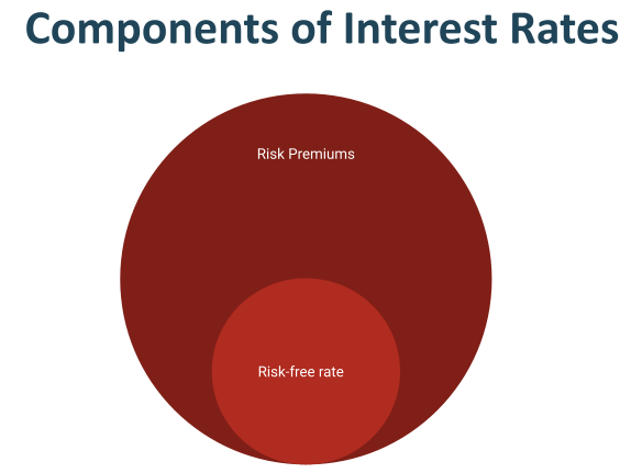
There are two main components to interest rates: the risk-free rate and risk premiums (Figure 5.3). The risk-free rate is the interest rate on a hypothetical investment that has no risk. The 3-month U.S. Treasury Bill is often used as a proxy for a risk-free investment because historically the U.S. government has never defaulted on its debt since the civil war. The risk-free rate is affected by inflation and the supply and demand for money. When the economy is strong, there will be greater demand for money and the risk-free rate will be higher. The federal government’s monetary policy can affect the supply of money and influences the risk-free rate. When unemployment is high and economic growth is slow, the Federal Reserve will increase money supply to decrease interest rates. Lower interest rates will encourage businesses to invest and consumers to spend more. When inflation is rising, the Federal Reserve will shrink money supply to increase interest rates to reduce consumption. Since investors must be compensated for the effect of inflation, the risk-free rate also rises and falls with inflation.
All investments and loans carry risks to varying degrees. The interest rates on these include the risk-free rate plus a risk premium. The risk premium is affected by four factors. The first factor is the overall risk averseness of investors. High confidence among consumers and businesses tends to reduce risk averseness and lower risk premiums. Uncertainty about the future will increase risk premiums. The second factor is the default risk of the borrower, which varies from borrower to borrower. Higher default risk leads to a higher default risk premium. The third factor is maturity risk. The longer the term of an investment or loan, the higher the maturity risk premium. The last factor is liquidity risk. Liquidity refers to the ability to sell an asset for cash quickly without depressing its value. Let us see how this interest rate model works in real life. A borrower with a higher credit score (therefore lower default risk) will be able to get loans at lower interest rates. In general, the interest rate on a 15-year mortgage is lower than the interest rate on a 30-year mortgage because the 15-year mortgage has lower maturity risk. The rule of thumb is that higher risk results in higher interest rates. This rule applies to investments as well as loans. If you invest in higher risk securities, you should demand a higher expected return. Beware of investments that promise high return with low risk. Financial markets are highly competitive and investments that sound too good to be true, usually are bad. Investors with limited wealth and income are least suited to invest in high risk investments, even if the high returns appear attractive.
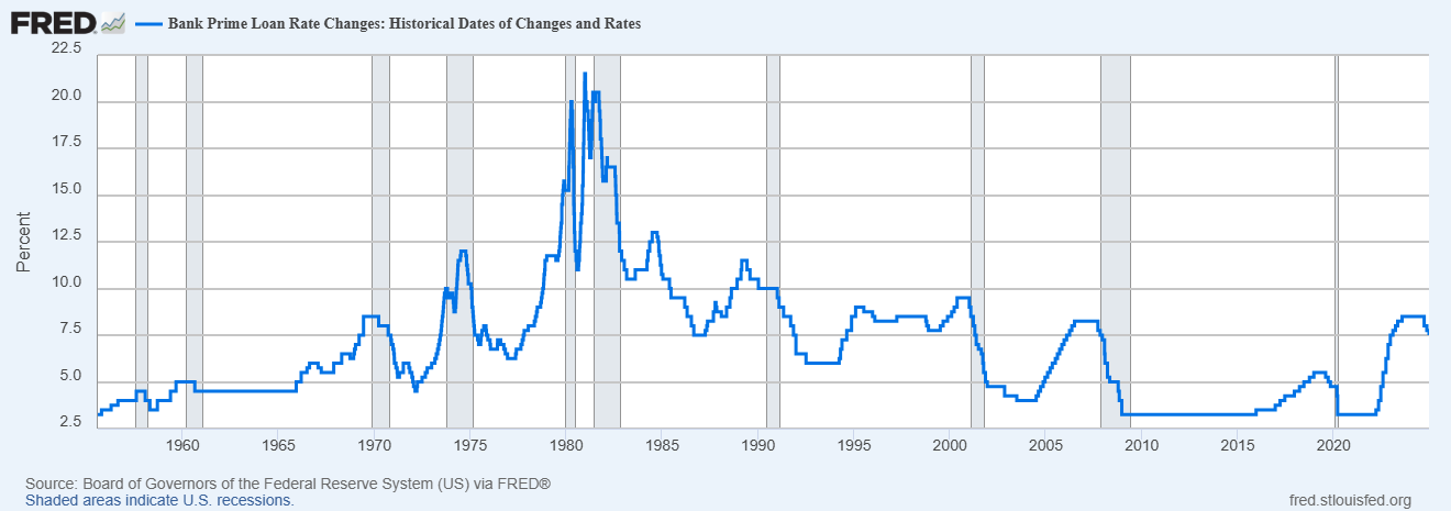
Some interest rates are fixed, which mean the rates remain constant for the duration of a loan or an investment. Examples include certificates of deposits, fixed rate mortgages, and many government bonds. The fixed rates provide predictability and makes financial planning easier but have less flexibility. Variable interest rates fluctuate based on market conditions. Examples include credit cards, adjustable rate mortgages, and savings accounts. Many variable rate loans such as credit cards and adjustable rate mortgages are tied to the Prime Rate. The Prime Rate is the lowest interest rate the largest banks charge their most creditworthy large customers. The interest rates on consumer loans are stated as Prime Rate plus a margin. For example, the interest on an adjustable rate mortgage is Prime Rate plus 3 percent. In March 2020, the Prime Rate was 3.25 percent, meaning the interest rate on this mortgage would be 6.25 percent. In July 2023, the Prime Rate was 8.5 percent, meaning the interest rate on this mortgage could go up to 11.5 percent, increasing the monthly payment significantly. We will discuss mortgages in more detail in a later chapter. The key takeaway here is that variable interest rates are less predictable. Many variable rate loans offer a lower initial interest rate than fixed rate loans, making these loans attractive. It is important to take into account potential rate increases when considering these loans. Historically, the lowest Prime Rate was around 3.25 percent and the highest was 11.5 percent in 1981 (Figure 5.4).
Whether you are saving for a house down payment, investing for retirement, or managing debt, interest rates play a crucial role. They influence every aspect of your financial life, from daily transactions to long-term goals. Understanding factors that affect interest rates and the different types of interest rates are important for personal financial planning.
Integrated Case 5
Applying Time Value of Money in Financial Planning
Blake Jackson had let her credit card balance grow to $3500 at the end of June. At an interest rate of 20 percent per year, the credit card balance can grow quickly. One of Blake’s short-term financial goals is to pay off the current balance within one year. She expects to be able to pay $1200 per month over the next two months as she will be working full-time over the summer. Once school begins in September, she will have to cut back her hours significantly.
Activities:
- What will the credit card balance be after the next two months, assuming interest will be computed at the end of each month and Blake pays $1200 per month? (Hint: interest per month = remaining balance x interest rate per year / 12. New balance = previous balance + interest per month – payment per month)
- How much will Blake need to pay per month starting in September if she wants to pay off the remainder of the balance in the next 10 months?
Chapter Five Summary
This chapter explains opportunity cost, time value of money, compounding, and various types of interest rates. Mastering these concepts provides a foundation for analyzing investments and loans.
Opportunity Cost
Opportunity cost is defined as the value of the next-best alternative when you make a decision. This means that every financial decision carries a cost beyond the direct monetary outlay. Recognizing opportunity costs helps individuals make more informed choices by considering what they are giving up.
Time Value of Money (TVM)
The core principle of time value of money is encapsulated by the saying, “A dollar today is worth more than a dollar tomorrow.” This is due to two primary factors:
- Inflation: The increase in the price of goods and services over time. Money held today will likely buy less in the future.
- Opportunity to Earn Returns: A dollar not spent today can be invested, earning interests, dividends, and capital gains, which allows it to grow to more than one dollar in the future.
TVM calculations are essential tools for analyzing investments, loans, and financial planning.
The Power of Compounding
Compounding is when the return earned or interest owed is added back to the investment or loan. This process, also known as interest on interest, allows balances to grow and accumulate over time at an accelerating rate.
Simple Interest vs. Compound Interest:
- Simple Interest: Assumes earnings are not reinvested. For a $1,000 investment at 10 percent per year, simple interest would yield $100 annually, totaling $200 over two years (new balance $1,200).
- Compound Interest: Reinvests earnings. The same $1,000 investment at 10 percent would yield $100 in Year 1 (new balance $1,100), and $110 in Year 2 (new balance $1,210).
The growth of money through compounding depends on:
- Time: The longer you invest, the more your money grows.
- Rate of Return: The higher the rate of return on an investment, the more your money grows.
- Compounding Frequency: The more often you reinvest, the more your money grows. Common frequencies include annually, quarterly, and monthly. Many consumer loans like credit cards and mortgages use monthly compounding, meaning unpaid interest quickly adds to the principal.
Time Value of Money Calculations and Spreadsheet Applications
Spreadsheet software (e.g., Google Sheets, Microsoft Excel) provides built-in functions:
- FV(): Computes the future value.
- PV(): Computes the present value, also known as “discounting.”
- RATE(): Computes the rate of return or interest rate per period.
- NPER(): Computes the number of periods (time horizon).
- PMT(): Computes the annuity payment amount per time unit.
Understanding Interest Rates
Types of Interest Rates
- Annual Percentage Yield (APY): Also known as the Effective Annual Rate (EAR), APY takes into account the effects of compounding when interest is computed more frequently than once per year. This makes it suitable for comparing investment products, as it reflects the true annual return.
- Formula: APY = (1 + (interest rate per year / compounding frequency per year)) ^ compounding frequency per year – 1.
- Annual Percentage Rate (APR): APR includes the total interests and fees related to the loan and is typically used for loan products. It provides a consistent basis for disclosing borrowing costs under the Truth in Lending Act (TILA). However, not all costs and fees are required to be included in the calculation of APR. Therefore, consumers still need to read the fine prints.
- Formula: APR = ((Fees + Total Interests) / Principal) / number of days in the loan x 365.
Financial institutions often advertise APY for savings to show higher returns and APR for loans to show lower initial rates, potentially misleading consumers without careful attention.
Components of Interest Rates
Interest rates are generally comprised of:
- Risk-Free Rate: This is the theoretical interest rate on an investment with no risk. The 3-month U.S. Treasury Bill is often used as a proxy. This rate is influenced by inflation and the supply and demand for money.
- When the economy is strong, demand for money increases, raising the risk-free rate.
- Monetary policy (e.g., by the Federal Reserve) affects money supply, influencing this rate.
- Risk Premiums: Additional compensation for various types of risk associated with an investment or loan. These include:
- Overall Risk Averseness of Investors: High confidence reduces risk premiums; uncertainty increases them.
- Default Risk: The risk that a borrower will not repay the loan. Higher default risk leads to higher default risk premium. Higher credit scores generally result in lower interest rates.
- Maturity Risk: The risk associated with the length of an investment or loan. The longer term an investment or loan, the higher the maturity risk premium. For example, 30-year mortgages typically have higher rates than 15-year mortgages.
- Liquidity Risk: The risk that an asset cannot be quickly sold for cash without losing value.
Fixed vs. Variable Interest Rates
- Fixed Rates: Remain constant for the duration of the loan or investment, offering predictability and makes financial planning easier. Examples include fixed-rate mortgages and certificates of deposit.
- Variable Rates: Fluctuate based on market conditions, often tied to a benchmark rate like the Prime Rate, which is the lowest interest rate large banks charge their most creditworthy customers. While variable rates may offer a lower initial rate, they are less predictable and can significantly increase monthly payments if the benchmark rate rises.
End of Chapter Questions
- Explain why a dollar today is worth more than a dollar tomorrow.
- Define opportunity cost and provide an example.
- Explain the concept of compounding in finance. How does it differ from simple interest?
- What are the three main factors that determine how much your money grows with compounding?
- Define Present Value (PV) and Future Value (FV) in financial calculations.
- Define an ordinary annuity and an annuity due. Provide an example for each type.
- When performing time value of money calculations using spreadsheet functions, what critical assumption does the software make about cash flows?
- Explain the importance of matching time units when using spreadsheet functions for TVM calculations. Provide an example.
- What is the difference between APY (Annual Percentage Yield) and APR (Annual Percentage Rate)?
- What are the two main components of interest rates?
- What is the risk-free rate, and what factors affect it?
- What four factors affect the risk premium component of interest rates?
- Explain the difference between fixed and variable interest rates, and provide examples for each.
- Why should investors be cautious of investments promising high returns with low risk?
- Jordan received a $2,000 graduation gift today and decided to invest it in an Individual Retirement Account (IRA), expecting to earn 11 percent per year. Compute the estimated value of this investment after 40 years, assuming no additional contributions.
- Sam has accumulated $8,000 in credit card debt with a 24 percent annual interest rate. If Sam commits to making minimum payments of $50 per month for 24 months and makes no additional purchases, Compute the remaining balance at the end of the 24 months.
- Jordan’s company offers a retention bonus of $15,000 if they stay for 3 years. A competitor is offering a $12,000 sign-on bonus today. If Jordan can invest money at an 8 percent annual return, how can they compare these two offers using present value, and which option is more financially beneficial today?
- Sam, currently 25 years old, wants to accumulate $1,500,000 by age 70 for retirement. Assuming an average annual investment return of 10 percent and no current savings, how much money will Sam need to save each month to reach this financial goal?
- A car dealer offers financing on a $35,000 car with monthly payments of $675 for 72 months. Compute the annual interest rate for this loan.
Appendix 5
Creating spreadsheet templates to perform time value of money calculations
This appendix assumes that you have moderate knowledge of spreadsheets, including the use of functions, formulas, and cell references. You can skip this appendix. It will not affect your ability to understand and master future chapters.
A template is a simple financial model. Despite its simplicity, some basic design principles still apply.
- Avoid hard coding numbers in formulas.
- Keep formulas readable.
- Be consistent in the model structure.
- Use color coding to emphasize user inputs and model outputs.
- Clearly label inputs and outputs.
- Minimize input errors.
- Validate input wherever possible.
To determine user inputs and model outputs, a spreadsheet designer conducts interviews with users to assess their needs and workflow. In this appendix, the purpose of the templates is to perform time value of money calculations. The input variables have been specified earlier in this chapter. We need to decide the format for the input variables. For example, should the user input return per time unit or input interest rate per year? This is a design decision. We decide to have the user input interest rate per year because that is the most common format interest rates are quoted.
Compounding frequency is another input variable. However, in our experience converting time units to compounding frequencies is not intuitive for some users. The template can do this conversion easily. The design decision here is to have the user input the time unit instead of the compounding frequency. To minimize input error, the template will use a drop down menu so the user can select the time unit.
The first template is to compute future value. Since this template is very simple, we will put all the elements on the same sheet. We use Google Sheets in this appendix. The first part of the template (Figure 5A.1) informs the user of the purpose of the template and the color codes.
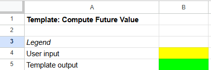
The second part (Figure 5A.2) contains the input area. This template is used to compute future value, therefore the input variables include:
- Time unit
- Interest rate per year
- Number of periods
- Annuity amount per period
- Present value
- An indicator with 0 for ordinary annuity and 1 for annuity due.
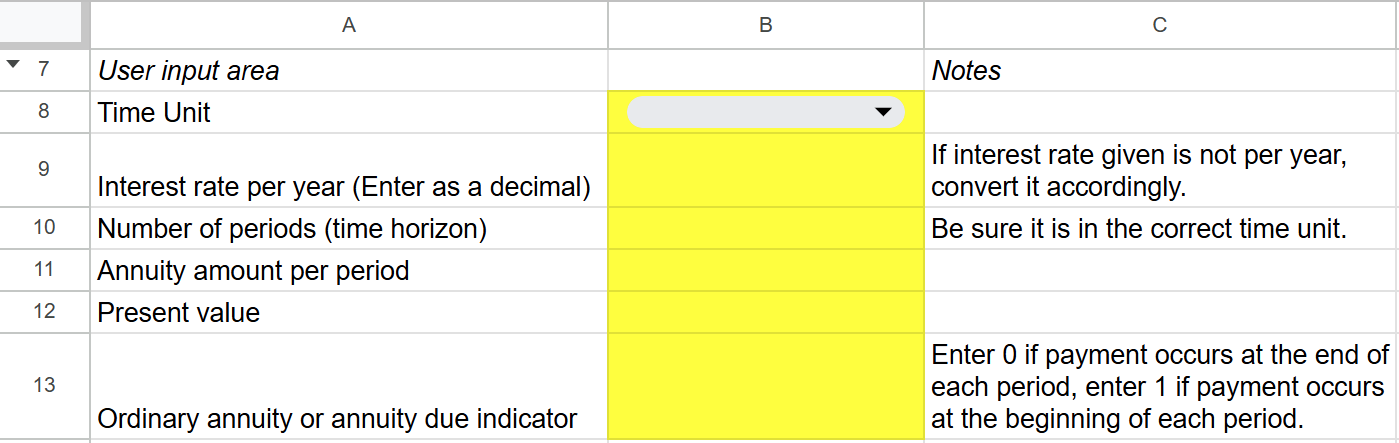
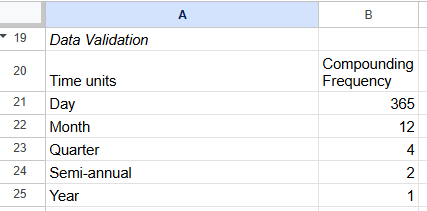
We include notes to help the user enter input variables in the correct format. Notice the input for cell B8 (time unit) is a drop down menu. The valid options for time units are included in the data validation area, Figure 5A.3.
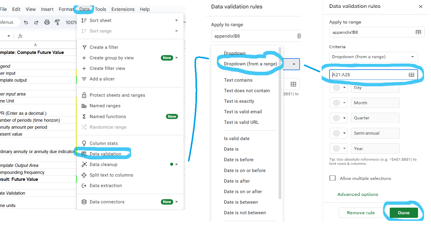
To implement this data validation rule, first select cell B8. Then choose [Data] from the top menu and [Data validation] from the submenu. From the Data validation rules menu, choose the option [Dropdown (from a range)]. Enter the range containing the time units, A21:A25. Select [Done]. See Figure 5A.4. If you do not use Google Sheets, the menu options will look different.
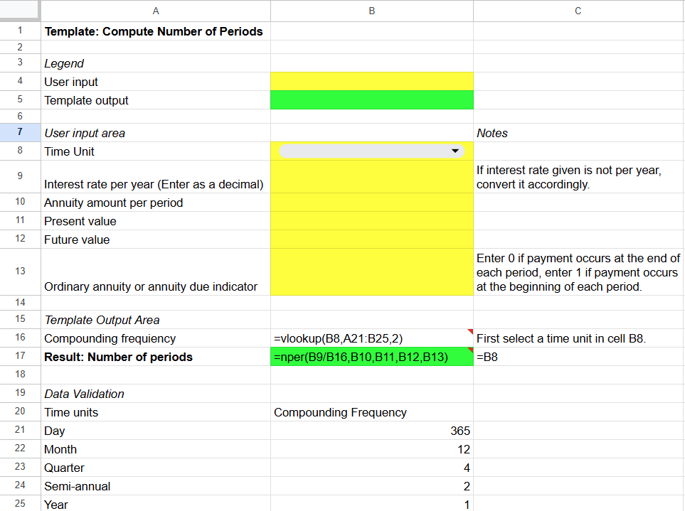
This template has 2 outputs. The first output converts the time unit into a compounding frequency. We did not color code this output because it is an intermediate calculation and not the final output of the template. Figure 5A.3 shows that the compounding frequency is specified next to the corresponding time unit. The compounding frequency is used to convert interest rate per year to the appropriate rate per period. This calculation is done in cell B16. We use the vlookup function to select the correct compounding frequency. The formula for cell B16 is ‘=vlookup(B8, A21:B25,2)’ (Figure 5A.5). Cell B8 contains the time unit selected by the user. Cells A21:B25 contains the time unit and the compounding frequency. The number 2 specifies that the compounding frequency is in the second column.

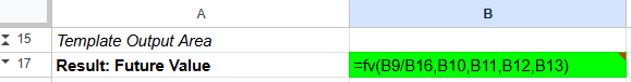
Cell B17 contains the output from this template which is the future value. The formula for cell B17 is =FV(B9/B16,B10,B11,B12,B13). This function is explained earlier in this chapter. In this template, cell references are used in the function instead of numbers (Figure 5A.6). By creating a template, you can use it to compute future values easily by changing the input variables.
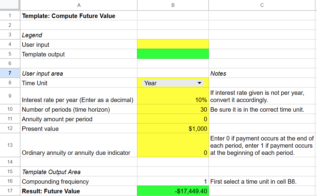
You can test your template using one of the examples in the chapter. Figure 5A.7 shows the template’s calculation for a $1000 investment at 10 percent per year over 30 years.
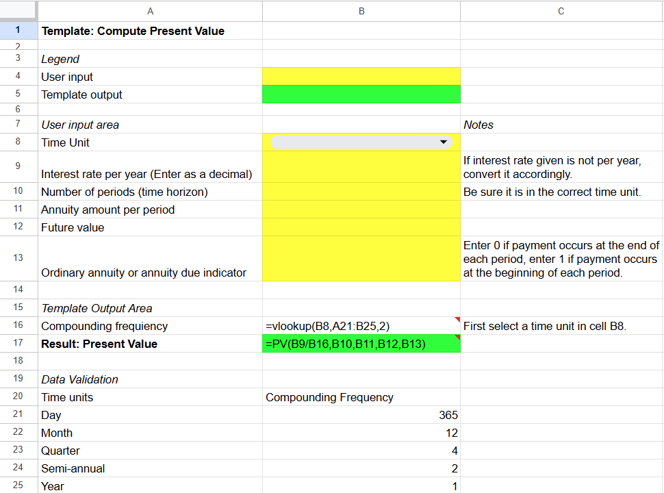
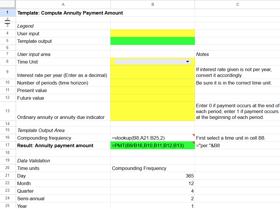
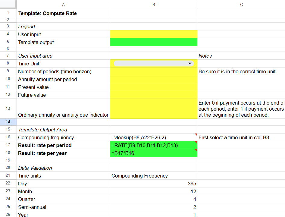
You can create similar templates for computing present value (Figure 5A.8), annuity payment amount (Figure 5A.9), rate (Figure 5A.10), and number of time periods (Figure 5A.11).
- An extensive discussion of how to use spreadsheets to create financial models is beyond the scope of this textbook. Appendix 5 shows you how to create simple templates to perform time value of money calculations. ↵
Opportunity cost is the value of the next-best alternative when a decision is made.
A rate of return is the net gain or loss of an investment including interests, dividends and capital gains or losses over a specified time period, expressed as a percentage of the investment's initial cost.
The expected return is the rate of return that an investor expects from an investment. It is not guaranteed. It is often based on long-term weighted average of historical returns.
Realized returns represent the actual gains or losses earned from an investment, expressed as a percentage.
The time value of money is a financial principle which states that a sum of money is worth more today than in the future.
Simple interest is calculated using on the principal and does not include compounding interest.
Future value is how much a sum of money will be worth in the future based on a specified interest rate.
Compounding frequency refers to the number of times interest is computed and added to the balance in each year.
A lump sum is a single payment made at a particular time with no repeat.
An annuity is a fixed amount of money paid or received at regular intervals over a finite interval.
An ordinary annuity is an annuity with payments occurring at the end of each period.
An annuity due is an annuity with payments occurring at the beginning of each period.
Discounting is the process of computing the present value of a future cash flow based on a specific interest rate.
A discounted rate is the rate of return used to determine the present value of future cash flows.
Discounted cash flow analysis is used to estimate the value of an investment or a company by discounting its estimated future cash flows to a present value based on a discount rate.
